Introduction to Minimax regret

I often get question about the meaning of minimax regret and how to calculate it, so here is a short introduction.

Online learning describes the world as a repeated game; for each round 1,ldots,T , the learner plays an action a_tinmathcal A , then nature plays a response x_tinmathcal X (perhaps even adversarially chosen given the player's action), and the player witnesses and incurs the loss ell(a_t,x_t) . How can we measure the preformance of the player? Very simple strategies of nature can insure linearly growing expected cumulative loss; even choosing x_t i.i.d from some distribution is sufficient. Instead, we try to control regret, mathcal R , which is the difference between her cumulative loss and the cumulative loss of the best action in some comparison class. That is,

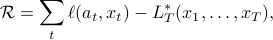
mathcal R = sum_tell(a_t,x_t)-L_T^*(x_1,ldots,x_T),

where L_T*(x_1,ldots,x_T)=min_a sum_tell(a,x_t) . Early work with a finite comparison class of size and arbitrary bounded loss function described algorithms that have regret upper bounds of 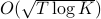O(sqrt{Tlog K}) with lower bounds that show that any algorithm can be made to suffer regret of the same order (e.g. weighted majority and many others).

There is a stronger notion of optimality where we guarantee achieving the best possible regret aganist all response sequence. For a single round game, the adversary can pick 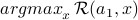$mathop{argmax}_x mathcal R(a_1,x)$ ; therefore, the player should chose a_1 to minimize this worst-case regret. For two rounds, nature at round plays assuming that the player will play the minimax response in round , and therefore the player at round 1 minimizes this maximum regret. 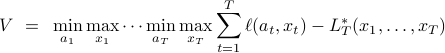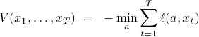Extending to rounds,the value, or minimax regret, is defined as

$V ~:=~ min_{a_1}max_{x_1}cdots min_{a_T}max_{x_T}quad mathcal R(a_1,x_1,ldots,a_T,x_T).$

Intuitively, this is simultaneously the minimum regret possible by the player and the maximum regret possible by nature. To evaluate the value, it is often convinient to write it out as a backwards induction. First, note that we can write the value as:

$V~=~ min_{a_1}max_{x_1}cdots min_{a_T}max_{x_T} sum_{t=1}^Tell(a_t,x_t)-L_T^*(x_1,ldots,x_T)$

$quad ~=~ min_{a_1}max_{x_1}ell(a_1,x_1)+min_{a_2}max_{x_2}ell(a_2,x_2)+ldots +min_{a_T}max_{x_T} ell(a_T,x_T)-L_T^*(x_1,ldots,x_T).$

where we have just moved terms around. It is then straightforward to check that recursively definite the value-to-go V(x_1,ldots, x_t) with base case

$V(x_1,ldots,x_{T}) ~=~ - min_{a} sum_{t=1}^T ell(a,x_t)$

and induction step

$V(x_1,ldots,x_{t}) ~=~ min_{a_{t+1}} max_{x_{t+1}} ell(a_t,x_t) + V(x_1,ldots,x_{t+1})$

will give the value for the base case of t=0 . One can think of the value-to-go V(x_1,ldots,x_t) as essentially the regret if responses of were played in the first rounds, then both players played optimally from then on. The reason that the optimal actions depends on the past is because L_T^* depends on them. We need to account for the difficulty in the comparator when playing actions this round, as always choosing hard actions (to make ell(a_t,x_t) large) may make L_T^* large and therefore regret small